Step-by-Step Flatness Symmetry

Add a ‘Flatness and symmetry physics QA’ object to your case.

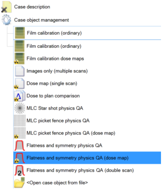
There are three types of objects: ‘Flatness and symmetry physics QA’ object can hold any number of images to be analyzed and uses the images directly. The ‘Flatness and symmetry physics QA (dose map)’ analyzes only a single image that will be converted into a dose map. ‘Flatness and symmetry physics QA (double scan)’ uses both portrait and landscape scan of the same film to avoid lateral scanner effect entirely.

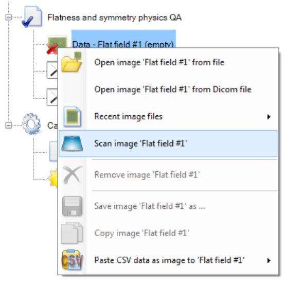
Acquire the image with the flat field exposure - either read it from file or scan it directly.

For automated image Registration select the fiducial tool and mark the fiducial positions at the star shot image as shown below. Any number of fiducials can be used to identify the isocenter. However, the minimum number to determine both x, y shift and rotation is 3 fiducials.

Tip: To move the fiducial marker , select it and either drag it with the mouse pointer or use Ctrl+Arrow keys. To delete a fiducial marker, select it and press Del key.

To change the fiducial type open the fiducial tool and select the wanted type.

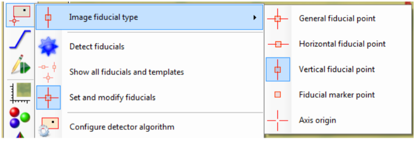
General fiducials are used to fit both a and y axis of the isocenter, Horizontal fiducials fit only the y coordinate.

When all fiducials are marked, select the tool “Flatness and symmetry physics QA” in the case tree.

The isocenter is automatically fitted to the marked fiducials as shown below.

Tip: Isocenter can fitted with other options using the fiducial fitter tooland selecting the wanted type of fit (see below).

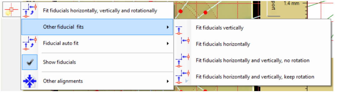
The flatness and symmetry tools automatically assigns the horizontal and vertical analysis path lines.

Use the button to configure analysis process including used analysis path lines as shown below.

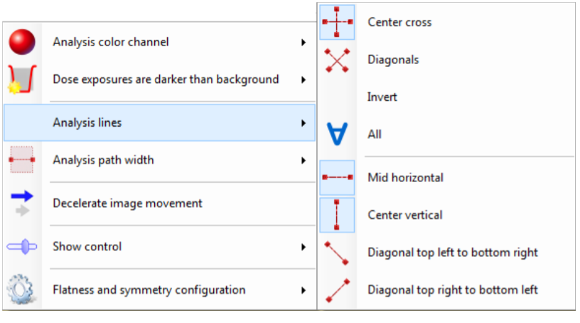
The detected results may depend on the average width of the chosen analysis path lines (average perpendicular to the path direction) and the color channel used to analyze the image data.

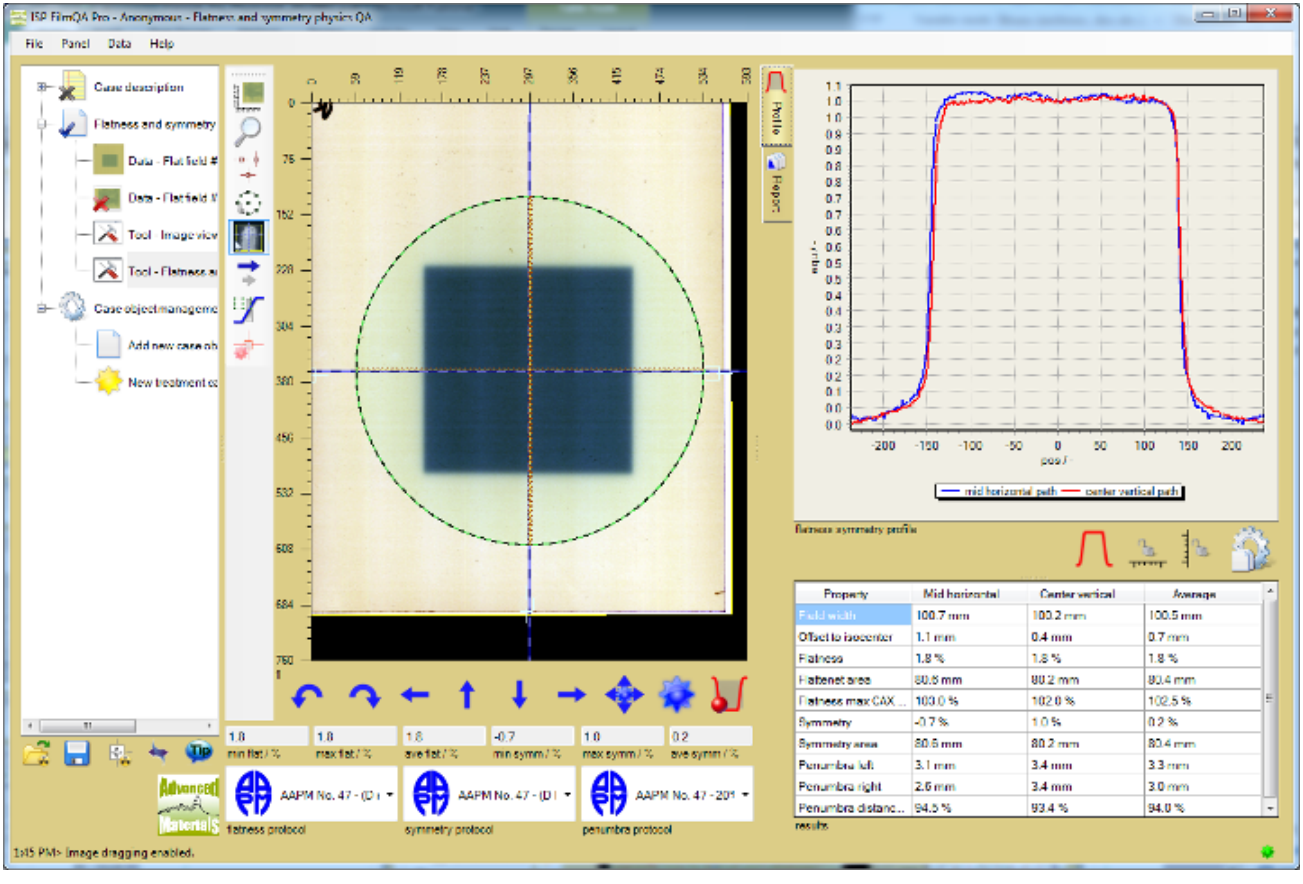
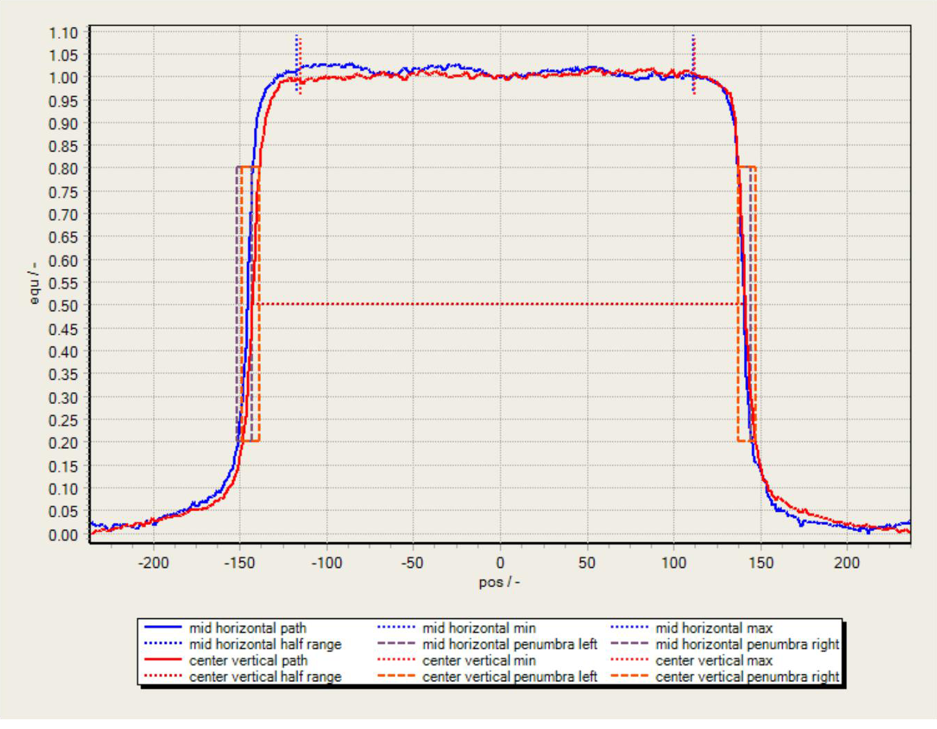
The profile tab at the right shows a chart of the profiles along the selected analysis path lines and a table with the numerical analysis data according to the selected analysis protocols for flatness, symmetry and penumbra (see bottom of the center section).

The profile data can be normalized in different ways, use the button to to select the normalization mode.

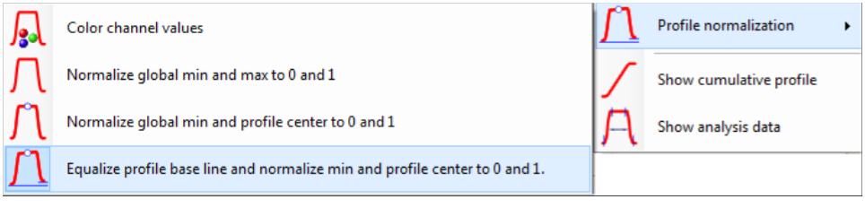
The maximum or CAX value can be normalized to 1 and the profile minimum to 0. If the base line of the profile is disturbed (left and right values are different) the base line can be equalized using a linear adjustment.

If show analysis data is selected, the flatness region as well as the penumbra areas are marked in the chart as shown below.

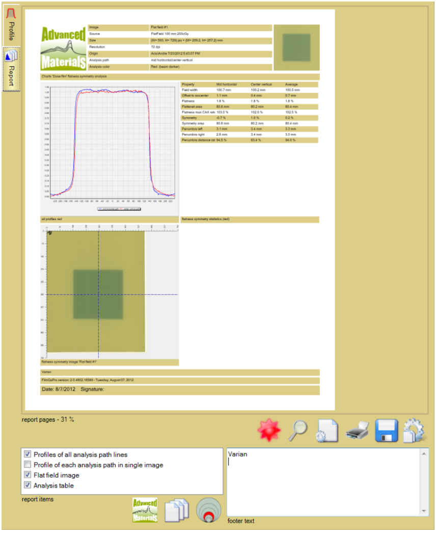
When the analysis is completed, select the report tab to summarize the results for the records.

Enable the items that should be included in the report and add the information to identify the test in the ‘footer text’ box.

watch the video